In this project I will perform a finetuning from scratch on Mistral 7B, particularly a QLORA, then compare the finetuned version and the base one making an example generation; and finally run the perplexity test to see the improvement after the training.
In a previous article, I performed a finetuning using a third-party provider, in this case, I will build the process from scratch so this code can be easily applied to any other dataset or model.
It’s important to notice that to perform this training I have used GPU, particularly the T4 from NVIDIA that can be used for “free” in Google Colab. In case of not being able to use any free provider or not having access to GPU, I recommend running a smaller model in the CPU.
Introduction
Before starting with the whole process, let’s see what are going to do and what we expect.
The idea of the project is to take a vanilla (Base) model and finetune it using a QLoRA method to be able to write Frankenstein inspired stories. After that, we will make an example generation to see by ourselves the difference in quality and finally perform a perplexity test to see which one is better.
Let’s unpack some of the concepts mentioned before:
What is a QLoRA
This is a specific type of finetuning for Neural Networks, and it’s a combination of two actions, Q (Quantization) + LoRA (Low-Rank Adaptation). I will explain both separately and then watch the combination:
For the next explanation I will assume some knowledge of Neural Networks, for reference and refresher check the next link, to make the article not too long, I will simplify the concepts but provide a reference in case of wanting to go deeper.
Quantization
In the world of AI, there are multiple types of LLMs, and one of the main characteristics of them, it’s the parameters, in this case for us for example, we are working with Mistral 7B, which means that it has 7 Billion parameters, which is not small by any means.
More parameters mean more space needed to store them, which at the end of the day means more costs. So we can go and use a smaller model so it will be lighter, but here we run into another issue the smaller the model, the more “stupid” the model is.
So the question that we can ask is: is there any way of compressing our existing model without losing [almost any] quality in the generation? The answer is yes, and this is call quantization.
The way this process works is by turning high precision values to make them lower precision values so they occupy fewer bytes (Space).
Reminder: 8 bits = 1 byte
Usually, most LLM are trained with float32 values, which means that each value is 32 bits, so 4 bytes, to have an idea of this a 1 billion parameter model will require 4 Gigabytes. But if we reduce the precision of these numbers we can save a lot of space, let’s see the for others:
| Precission | bits | bytes | Space needed for a 1B parameter model |
|---|---|---|---|
| float32 | 32 | 4 | 4 GB |
| float16 | 16 | 2 | 2 GB |
| int8 | 32 | 1 | 1 GB |
| int4 | 32 | 0.5 | 0.5 GB |
We can see the insane result that we can get with a quantization, of course, be aware of the reduction in quality due to this technique. In our case, we are going to use int4, the smallest one.
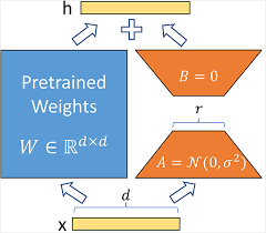
LoRA (Low-Rank Adaptation)
The other part of the equation in our process is going to be a technique called LoRA.
When we train our LLM we get a matrix, with the different weights of the Neural network, big models like Mistral 7B have really big matrixes, which is why during their training they require vast amounts of computing power (GPU) to handle all the operations.
When we want to re-train our model, like ourselves now, we don’t want to update all the weights and do all the calculations, we can only re-train the weights that matter, which will make our cost and computing needs way lower while having a great result.
The most famous visualization for LoRA is the next one:
Now, I just said re-train the weights that matter, but what exactly does this mean? This is a complex algebraic problem, but let’s give a simple example to understand:
Let’s imagine we have the next 3x3 matrix:

What we can see from this image is that the first and last columns are not “important” as they are not giving us information, we can get them by multiplying the second one by 2 (We get the first column) and by 0 (We get the third column).
So according to algebra this matrix has rank 1 and can be decomposed into the product of two other matrices size (3x1) and other (1x3). So we are going to update the weights that “matter”.
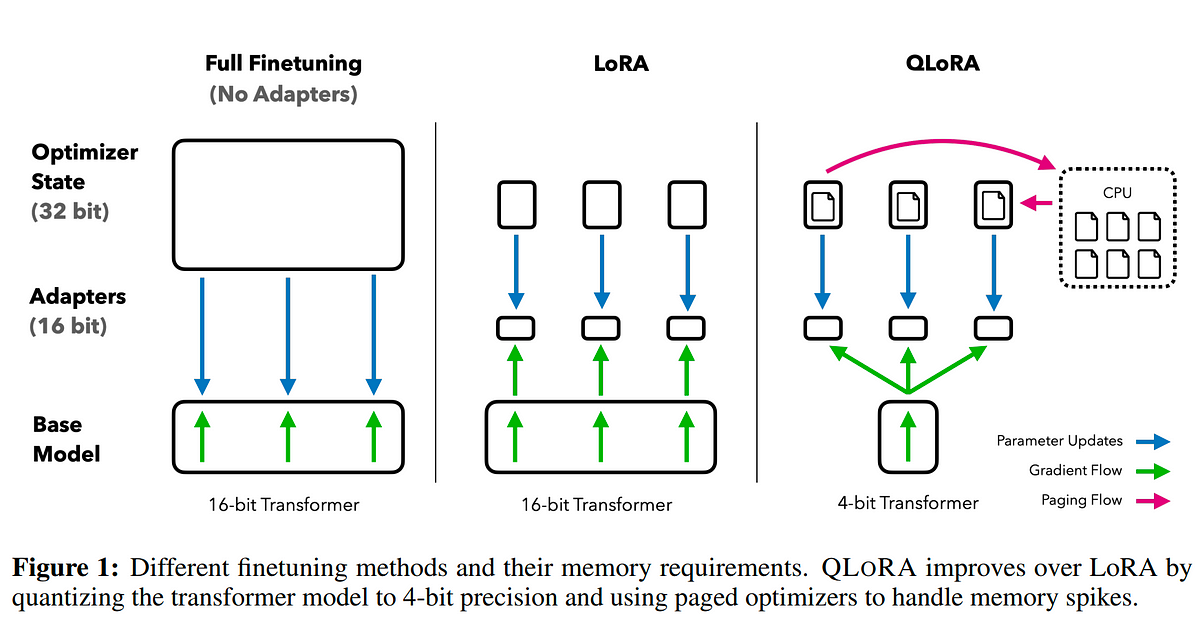
Now that we know these concepts we can combine them into QLoRA, the next diagram showcases all the steps:
Programming the QLoRA
Now that we have the idea in mind of what we want to do and also the main concepts, let’s start with the code.
Installing and importing
Let’s start by installing all the necessary libraries, most of the libraries that allow us to perform this process are from huggingface.
!pip install -qU bitsandbytes transformers peft accelerate datasets pandas torch
We also want to import the libraries and set some parameters such as the seed to be able to reproduce the exact same output.
import random
import torch
import pandas as pd
from datasets import Dataset
import peft
from transformers import AutoTokenizer, AutoModelForCausalLM, BitsAndBytesConfig
def set_seed(seed=42):
    random.seed(seed)
    torch.manual_seed(seed)

set_seed()
Exploring the data
The dataframe we are going to use it’s a csv file with sentences from Frankestein, we can use any other text file we want but be aware of preprocessing the data, the cleaner, and wider our scope the data the better.
In the training process, data is critical. Garbage in, garbage out.
df = pd.read_csv("frankenstein_chunks.csv")
The data in this case is clean, but in case of using some other data is always useful to check it:
print("Dataframe Info:")
print(df.info())
print("\n")
print("Dataframe Description:")
print(df.describe())
print("\n")
print("Number of unique values in each column:")
print(df.nunique())

print(df.isnull().sum())
Also, we are going to split the data into a training set and a test set:
from sklearn.model_selection import train_test_split
train_df, test_df = train_test_split(df, test_size=0.2)

train_dataset = Dataset.from_pandas(train_df)
test_dataset = Dataset.from_pandas(test_df)
Tokenizing
This step is the longest one as we have to turn into tokens the information, to know more about what tokenizing is, as well as how to perform it, I recommend reading my article finetuning for text-SQL where I explained in detail and provide the code to do this.
First, we specified the model (type the model you want to use):
model_name = 'mistralai/Mistral-7B-v0.1'
Now we are going to download the model to perform the training and to use it, the model it’s in huggingface, so beware that you might get problems if you are not authenticated into hugginface, and in some models, if you don’t accept the terms and conditions. To make this log we need to generate a huggingface token and run the next code:
from huggingface_hub import login

login(token="<HF_API_TOKEN>")
With this solved we can get the model and perform the quantization that we explained before, earlier I said I would use the int4 as is the smallest, but it’s not exactly true (Sorry), we will use the so-called “nf4”, the Normalized float 4 bit, but the size applies the same.
quant_config = BitsAndBytesConfig(
    load_in_4bit=True,
    bnb_4bit_use_double_quant=True,
    bnb_4bit_quant_type='nf4',
    bnb_4bit_compute_dtype=torch.bfloat16,
)
model = AutoModelForCausalLM.from_pretrained(model_name, quantization_config=quant_config)

print(f"Running on: {torch.device("cuda" if torch.cuda.is_available() else "cpu")}") # It should be cuda if you are using colab with T4
Now we just going to define the parameters of the LoRA training and tokenize the train and test sets defined before, in this project, I will not enter into how all the parameters in the configuration depend on experience and trial error.:
from peft import prepare_model_for_kbit_training, LoraConfig, get_peft_model

model = prepare_model_for_kbit_training(model)
config = LoraConfig(
    r=32,
    lora_alpha=64, # This number is usually double the parameter "r".
    lora_dropout=0.05,
    task_type="CAUSAL_LM",
)

def tokenize_function(examples):
    return tokenizer(examples["text"])

model = get_peft_model(model, config)
tokenizer = AutoTokenizer.from_pretrained(model_name)
tokenized_train_dataset= train_dataset.map(tokenize_function, batched=True)
tokenized_test_dataset = test_dataset.map(tokenize_function, batched=True)
Base Model Performance
Now we have everything ready, so before starting, let’s see how the base model generates without training. I will create first a function to generate the result, for that we have to also do the decoding of the result.
def generate_text(prompt):
  device = "cuda"
  inputs = tokenizer(prompt, return_tensors="pt").to(device)
  outputs = model.generate(**inputs, max_new_tokens=100)
  output = tokenizer.decode(outputs[0], skip_special_tokens=True)
  return output
Let’s see what a model without training generates:
base_generation = generate_text("I'm afraid I've created a ")
print(base_generation)
Result (Base Model) I’m afraid I’ve created a 2000-level problem with a 100-level solution. I’m a 2000-level problem. I’m a 2000-level problem. I’m a 2000-level problem. I’m a 2000-level problem. I’m a 2000-level problem. I’m a 2
This is not the result we are expecting, so let’s train the model. But before starting let’s run the perplexity test, we will explain what it is in the last section of the article:
def calc_perplexity(model):
  total_perplexity = 0
  for row in test_dataset:
    inputs = tokenizer(row['text'], return_tensors="pt")
    input_ids = inputs["input_ids"]

    with torch.no_grad():
        outputs = model(**inputs, labels=input_ids)

    loss = outputs.loss
    perplexity = torch.exp(loss)
    total_perplexity += perplexity

  num_test_rows = len(test_dataset)
  avg_perplexity = total_perplexity / num_test_rows
  return avg_perplexity

base_ppl = calc_perplexity(model)
print(f"The perplexity score is: {base_ppl}")
The result is 8.9732
Finetuning
Now we can train the model, this process can take from 15 min to 45 min. Let’s start the process, thanks to transformers we can do it in a few lines of code:
import transformers

tokenizer.pad_token = tokenizer.eos_token
model.config.use_cache = False

trainer = transformers.Trainer(
    model=model,
    train_dataset=tokenized_train_dataset,
    args=transformers.TrainingArguments(
        warmup_steps=2,
        fp16=True,
        logging_steps=1,
        save_steps=200,
        output_dir="outputs",
        per_device_train_batch_size=2,
        num_train_epochs=2,
        learning_rate=2e-5,
        optim="paged_adamw_8bit",
    ),
    data_collator=transformers.DataCollatorForLanguageModeling(tokenizer, mlm=False),
)

trainer.train()
Now we have the model trained and ready to use.
Final Result
Let’s repeat the generation step and see the result:
ft_generation = generate_text("I'm afraid I've created a ")

print("Finetuned generation: " + ft_generation)
Result (Finetuned) I’m afraid I’ve created a monster, one whom you are powerless to oppose, and he will be a constant menace to your family and every other family on the face of the earth. “I have made him with another’s specs, and my own hands are unclean. Yet it is well I have done this deed; for now, am I released from the curse which I shall have brought on my family.
Which is an amazing improvement in the result, making sense and good quality.
Perplexity Score
Now we can repeat the perplexity test in the finetuned model and compare results:
ft_ppl = calc_perplexity(model)
print("Base model perplexity: " + str(base_ppl))
print("Finetuned model perplexity: " + str(ft_ppl))
Compared to the non-finetuned version we get (A lower number is better):
| Model | Perplexity Socore |
|---|---|
| Base Model | 8.9732 |
| Finetuned version | 6.7407 |
After finishing all the generation and the improvement by doing a finetuning, as a footer note, I will make a quick explanation of the perplexity test:
Perplexity test
Perplexity (PPL) is one of the most common metrics for evaluating language models. It is defined as the exponentiated average negative log-likelihood of a sequence, calculated with exponent base e.
Given a model and an input text sequence, perplexity measures how likely the model is to generate the input text sequence. As a metric, it can be used to evaluate how well the model has learned the distribution of the text it was trained on. Note that the output value is based heavily on what text the model was trained on. This means that perplexity scores are not comparable between models or datasets.
This was all about this QLoRA training for Mistral 7B and testing.
Thanks for reading!